[Engineering] Squircle

This article is aimed to help you implement the Figma’s corner smoothing effect step by step.

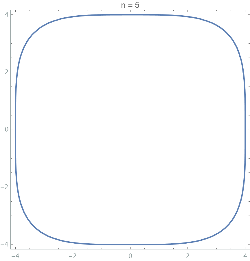
In design, rounded rectangle are a very common geometry used to enhance visual effects. Since iOS7, Apple proposed a new type of rounded icon that provide “pop” visual effect with something subtle around the corner. Initial reversing work comes from Marc Edwards, which reveals that this kind of contour might be governed by Superellipse $(\frac{x}{a})^n + (\frac{y}{b})^n = 1 $ with $n>2$

However, it not true for what iOS really does. After many efforts, it seems that the iOS-style corner is made of a combination of cubic Bézier curve and arc segment. The blog from Figma proposed a method that how to parameterized the smooth. With the value varies between [0, 1], the corner varies from a full arc to Bézier curve. Moreover, it could also apply to the corner with arbitrary angle rather than the 90-degree corner. The exposition on the mathematical theory in the original blog is sufficient, but it is obscured by ornate rhetoric, which can leave readers who wish to delve deeper into its mathematical principles rather perplexed. This article mainly focuses on the theoretical details proposed in the original blog and provides detailed mathematical formulas for each section, allowing readers to easily implement them in code based on these formulas.

0x00 Prerequisite:⌗

1. The definition of Bézier curves：

   • Here is a good introduction on Bezier for beginners.

2. Basic linear algebra:

   • A basic concept on affine transformation.

0x01 Mathematics Perspective⌗

Comparing two different kinds of rectangle, the squircle feels not as much abrupt as normal rounded rectangle at the joint between line and curve. This aesthetic comes from what is called continuation, in more specifically and mathematically speaking, Curvature Continuation. The necessary way to derive such a squircle is keeping the curvature continuation at the joint. Let’s begin from the basic idea behind the squircle.

But it’s far from enough to modeling a squirecle with the only condition mentioned above, since there are infinite curve combinations if specific curve form is not given. Considering simplicity in both mathematics and practice, Bezier curve (Cubic Bezier is enough for most scenarios) and circle, the most common and powerful tools in both engineering, computer graphics and 2D design, are adopted.

In fact, the original author show his idea from a mathematical perspective, where he assumes an continuous curvature profile, and he try to get the final integral curve by the given curvature equation. The result curve is called Clothoid, which is too complex and not in closed formed, far beyond out of our scenario.

Since the most curves can be given by a elementary function is already curvature continuatous itself. The only thing need to be done is having the value of curvature of both segments equal at their joint. Just recall that the condition of derivable or continous function you have learned in your high school.

0x02 Components⌗

Squircle corners are composed of an arc (part of circle) and two cubic Bézier curves at each end symmetrically. The proportion of Bézier curves included is controlled by a parameter, namely the smoothing. The smoothing ranges from 0 to 1. The larger the value, the longer Bézier curves are. When the value is 1, the arc part vanishes. When the value is 0, the arc is tangent with this angle, as the ordinary rounded angle used to be. As the smooth becomes larger, the length of arc part becomes less until smooth value is 1. Here is an illustration.

0x03 Math Foundation⌗

This section gives the sufficency condition for the curvature continuation at each joint without too much detail.

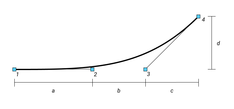
As the figure shows, the point 1 and point 4 are the end points of cubic Bezier and the point 2 and 3 are its control points. If we want get a continuous curvature profile for our smoothing curve, two constraints are held at the same time:

Constraint 1⌗

$If$ $P_1$, $P_2$ and $P_3$ are collinear, $Then$ $\kappa_{p_1}(0)=0$ $\implies$, $Then$ the curvature continuation is held between straight line part and the Bezier part

• $Proof:$

We know that the curvature of parameterized curve is

$$\kappa(t) = \frac{\left| B’(t) \times B’’(t) \right|}{\left| B’(t) \right|^3}$$

Given the cubic Bezier $B(t) = (1 - t)^3 \cdot P_0 + 3 \cdot (1 - t)^2 \cdot t \cdot P_1 + 3 \cdot (1 - t) \cdot t^2 \cdot P_2 + t^3 \cdot P_3 $

The curvature of cubic Bezier at $P_0$ ($t = 0$) is

$$\kappa_{p_1}(0) = \frac{\left| B’(0) \times B’’(0) \right|}{\left| B’(0) \right|^3} = \frac{\left| \left(6 \left(P_1-2 P_2+P_3\right)\right)\times \left(3 P_2-3 P_1\right)\right| }{27 \left| P_1-P_2\right| {}^3} $$

When $P_1$, $P_2$ and $P_3$ are collinear, the cross product of the numerator term equals $0$, so that $\kappa(0) = 0$ at $P_1$.

Amazing!

Constraint 2⌗

$If$ $P_1$, $P_2$ and $P_3$ are collinear $and$ $b = \frac{2}{3} \frac{(c^2+d^2)^\frac{3}{2}}{dR}$ $\implies$ $\kappa_{p_4}(1) = \frac{1}{R}$, $Then$ the curvature continuation is held between the Bezier part the Bezier part and the arc part.

• $Proof:$

Once we get the conclusion that $P_1$, $P_2$ and $P_3$ are collinear, we can put the curve at a special coordination for the further examnation. As above figure shows, we can simplify the representation of Bezier curve by the scalar $a$ $b$ $c$ and $d$ rather than using the vector $P_1$, $P_2$ and $P_3$, which reduces the complexity dramatically.

So when we put the curve at $P_1=(0, 0)$, and then $P_2=(a, 0)$ $P_3=(a+b,0)$ $P_4=(a+b+c,d)$ with respect to $a$, $b$, $c$ and $d$. Bezier curve $B(t)$ can be simplified as

$$ B(t) = ( t^3 (a+b+c)+3 (1-t) t^2 (a+b)+3 a (1-t)^2 t,d t^3 )$$

then the curvature at $P_4$ is

$$\kappa_{p_4}(1) = \frac{\left| B’(1) \times B’’(1) \right|}{\left| B’(1) \right|^3} = \frac{|(3c,3d) \times (6c-6b,6d)|}{|(3c,3d)|^\frac{3}{2}} = \frac{18|bd|}{|(3c,3d)|^\frac{3}{2}} = \frac{1}{R}$$

$deriving$

$$b = \frac{2}{3} \frac{(c^2+d^2)^\frac{3}{2}}{dR}$$

Smoothing Parameterized⌗

How we to control the visual effect of smoothing?

1. Intuitively, we would like a form with respect to $s \in [0, 1] \mapsto $ $Shape[a,b,c,d]$, saying that we could compute a corresponding set of $a,b,c,d$ from a given $s$.

2. Besides $s$, it should also be a map with respect to the arc part radius $R$. Written as $[s, R] \mapsto$ $Shape[a,b,c,d]$

3. The map must be invertable so that we could deal with the maximum smoothing value that corner could be.

Let’s explain each of these individually.

Picture the following, imagine we increase $s$ from 0 for all the three angle of an equalateral triangle at the same time with equal rate, the Bezier part will consume all sides with equal rate. What’s the smoothing angle looks like as the value increasing? And what’s the maximum value going to be? If the initial radius is relatively small, $s$ could be 1. But If the initial radius is larger, the Bezier part will consume the straight line before the parameter is going to be 1, because the side of triangle has no more room for angle being smoothing. So the map must be with respect to $s$ and $R$, namely $ s, R \mapsto$ $a,b,c,d$. As mentioned above, for larger $R$, the valid range of $is$ cannot come to 1. How we resolve the maximum value of $s$? What we only need to do is let the map be invertable. Then by giving the maximum room for consuming of each single angle, we can calculate $s$ by $Shape(a,b,c,d, R)$ $\mapsto$ $s$.

For a normal rounded corner, if the angle is $\theta$, then the segments consume of the edge is $\frac{R}{\tan{\frac{\theta}{2}}}$ = $R\sqrt{\frac{1+\cos\theta}{1-\cos\theta}}$, keep it simple as much as possible, we just define the squircle corner consume edge is $$ q=(1+s)R\sqrt{\frac{1+\cos\theta}{1-\cos\theta}} $$

Above form meet the 1, 2 and 3 at the same time.

Conclusion⌗

To get the curve with desired curvature profile, it’s necessary to make $P_1$, $P_2$ and $P_3$ collinear and hold $b = \frac{2}{3} \frac{(c^2+d^2)^\frac{3}{2}}{dR}$. In the next section, We will talk about how to code this step by step.